

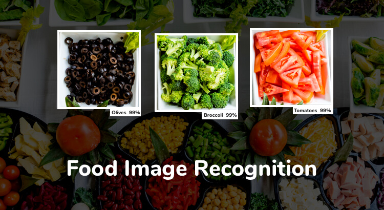
The field of image processing has progressed so much in the recent past that most of our customer inquiries for camera-based mobile applications now include some kind of image processing. One of them was to build a food image detection module to detect multiple food items from a mobile camera image and mark their positions. The following post details the various stages of our research and how we eventually built a highly accurate food image detector.
Establishing the Accuracy Metric
The first major step in executing any artificial intelligence project is to establish the success metrics early in the development cycle. Since object detection is a well-known machine learning problem, we knew what that metric would be—Mean Average Precision or mAP, the standard metric used to measure accuracy.
Let's have a look at how this metric works. Consider an image in which you have already annotated objects with bounding boxes. The measure of the accuracy of an object detector is how well this particular image gets mapped to predicted bounding boxes. (If you are not familiar with bounding boxes, please take a look at the TensorFlow object detection repository to understand the concept.)
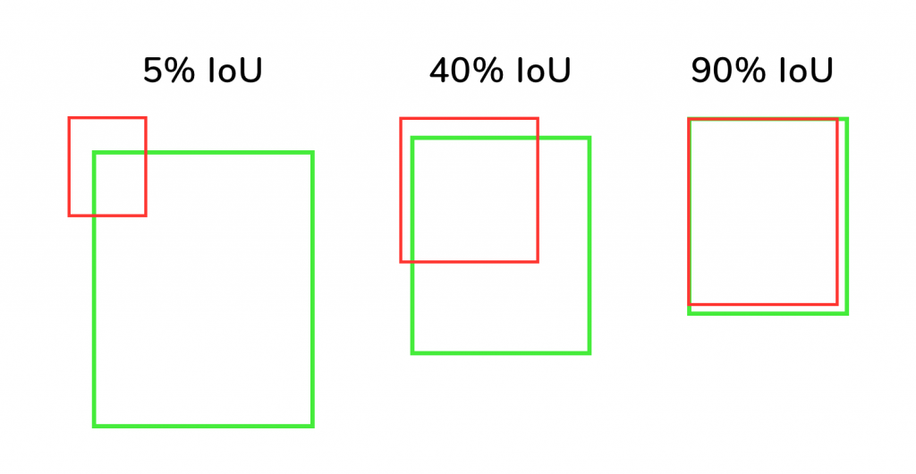
To classify a predicted bounding box as correct, we need to set a criterion. A commonly used metric for this is Intersection Over Union (IoU). To get the IoU value, we have to compare the predicted box and the original bounding box and find the area of overlap and the area of union.
Area of overlap = Number of pixels common to both the boxes
Area of union = Total number of pixels combining both the bounding boxes
The area of overlap divided by the area of the union gives you IoU.
IOU = Area of overlap / Area of union
You can understand more about IoU from the below image. It depicts the original bounding box in green and the predicted bounding box in red. For a predicted bounding box that is closest to the original bounding box, IoU will be more than 90% as shown in the rightmost image.
Now, there are a few calculations to be done before we get to Mean Average Precision.
First, we need to fix a threshold value for IoU above which the predicted box can be classified as correct. IoU is a fractional value, ranging anywhere from 0 to 100% (in absolute terms from 0 to 1). Let’s select the threshold IOU as .50 in absolute terms, that is, every box with an IoU greater than .50 will be considered as a correct prediction.
The next step is to find the precision values for the selected IOU of .50. In other words, we have to find the precision value by considering all the bounding boxes with an IOU greater than .50. Precision is a measure that conveys what proportion of positive identifications was actually correct.
Precision = Number of true positives / Number of predicted positives
True positives are images that were correctly predicted by the model. Predicted positives mean all the images that were predicted as positive by the model. Predicted positives will also include the images that the model thought were positive but was originally negative.
The average of all the precision values obtained by considering all the IoU values from .50 to .95 gives you the Mean Average Precision. To be more specific, we have to find the precision values by fixing IoU as .50, .55, .60… up till .90 and then find their average.
Now, that is too simplified an explanation—there is more to mAP than just calculating it for one specific scale or size of objects. But the above explanation should point you in the right direction in your research. A great example can be found in Microsoft’s COCO dataset GitHub repository. Now that we knew which standard to use for accuracy measurement, we moved to implementation.
Finalizing the Architecture
The field of object detection is still an evolving one, and several deep learning architectures with varying strengths are available to build an object detector. We considered the following factors while finalizing the architecture:
- In our case, the frames had multiple detection targets. Most architectures have a limitation when it comes to multiple detection targets in the same image.
- Speed and accuracy of detection.
- We wanted to stay within the product development budget.
- Support for a large number of labels. After much refining and deliberation, the least number of labels we could arrive at for a good food image detector was 280. All the currently available architectures lose on accuracy as the number of labels increases.
Most recent advancements in object detection have all been with variations of R-CNNs or Regions with CNN features. More details about the first iteration of RCNN can be found in the paper titled “Rich feature hierarchies for accurate object detection and semantic segmentation” by Ross Girshick et al.
R-CNNs solve the problem of low detection speed of classical CNNs using a region proposal network before the CNN layer. What this means is that, instead of feeding every possible slice of an image to CNN for detecting an object, R-CNNs feed only the regions proposed by the region proposal networks to CNN. In the initial iterations of R-CNN, proposing regions was done through a predefined algorithm called selective search. Later iterations improved on this by using neural networks for region proposals.
The state-of-the-art architecture when it comes to R-CNNs is the Mask R-CNN. Along with bounding boxes, Mask R-CNN is capable of providing a mask of the object, literally marking the boundaries of an object for clear detection.
Another important architecture in this domain is the Faster RCNN, which works similarly but lacks the ability to provide boundary marked output. Mask-RCNN is an extension of Faster RCNN with a branch added for detecting the object masks as well.
We tried both Mask R-CNN and Faster RCNN and found that their accuracy was comparable. The only advantage of Mask R-CNN is its ability to draw the boundary masks. But for the network to output those masks, we had to train it with the masks as well, which proved to be tedious. Since we were working on a tight deadline, we were short of time for data generation and training. Hence we decided to go with Faster R-CNN for this project.
Once we started working more with Faster R-CNN, we realized one of its limitations (not just R-CNN’s but that of every object detector currently available). The accuracy was closely tied to the number of labels and this went down as the number of labels increased. Since we had about 280 labels that could not be cut down, we started looking for alternatives. One of them was to use Faster R-CNN only to determine if an object was a food, crop the image, and then use a second image classification network like Inception-v4 on the cropped image. This had two advantages:
- Unlike object detection, which is still evolving, image classification is a mature field. Architectures such as the well-known Inception-v4 can provide great accuracy even with a large number of labels.
- Faster R-CNN only had to deal with two labels, which meant that it could perform optimally.
At this stage, this was merely speculative as we lacked real evidence. So we decided to try both approaches and measure the accuracy of the system.
End-to-End Detection
The idea was to use the same network architecture to detect the objects, mark them, and classify them by labels. For the experiment, we trained with 87000 images using TensorFlow Faster RCNN implementation. The highest accuracy which we could achieve was a mAP score of .427 with some hyperparameter tuning.
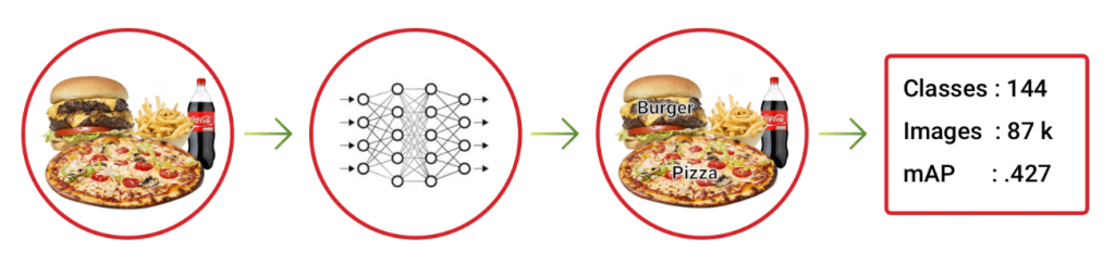
End-to-end detection: Single network architecture for detecting and classifying food
Detect–Classify Approach
In this approach, we used a Faster R-CNN network to train the food detector. This network only had to detect an object as food and draw a bounding box around it. So the training data for this network only had images with bounding boxes tagged as food and not the original set of labels. This model was followed by an image classification model, which used the cropped bounding boxes as the input and tried to classify them into 144 labels. The image classification model used was Inception-v4. We experimented with the same 87000 images and achieved a mAP score of .8 with a bit of hyper-parameter tuning.
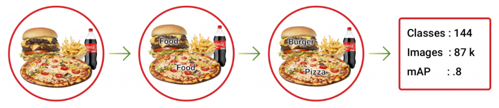
Detect–classify approach
After the experiments, it was clear that in our case a multi-stage system with a detector model and classification model performed better.
Collecting Data and Preparing for Training
The bulk of the effort in any artificial intelligence project is in collecting data and training the architecture. It is simple to train and test a network with a limited amount of data, but taking the model to production needs significant effort. In our case, because of our prior experience with image processing, we had access to many in-house tools that made tagging easier for us. There are services like AWS Mechanical Turk that assist in training, but we were trying to do this with as little manual effort as possible. This does not mean there was no manual effort; these tools and techniques work only after significant effort has gone into manual filtering and marking regions.
Some of the techniques and data sources which we used in this endeavor are given below:
- Recipe websites can be a source of food image training data. The data is not bounding box-tagged, but with some nifty tricks, you can generate bounding box data from them using pre-trained object models. Since the images are from recipe websites, you already know what the image contains. So all you need is to draw a bounding box around the objects using generic object detector networks and name them using the source information. But, first, check the licensing policies. Many websites prohibit the use of images.
- Some of the pre-trained object detection models available in the TensorFlow detection model zoo can detect popular food items like pizza and burgers. These models were also used to generate bounding box data.
- With auto-generation of bounding boxes, there should be a manual verification at some point before using training data. This manual verification can be sped up to an extent using simple scripts that pop up images with accept reject options. These scripts will make the verification faster than manual opening and selecting.
- OpenCV image processing library can be of great help in building tools to generate training data. Some of our in-house tools were implemented using simple background subtraction and contour detection techniques. Of course, it may not make sense to develop the whole suite of applications just for one project, but such tools can be of great help if you anticipate a lot of effort in the future.
In spite of all these options, we still had to put in significant manual effort to mark the regions accurately. But it would be safe to say that these helped us to increase training data availability by at least a factor of 100.
Conclusion
With our architecture, we managed to achieve
From our experience, at this point in the evolution of the image processing, if your project needs a large number of detection labels, it is better to use an object detection network along with an image classification network rather than an end-to-end network. The field is rapidly evolving and new models could make these tips obsolete, but just like the tools which we developed in our earlier endeavors helped here, the knowledge gained during the process will help reduce the time to production.