


A large variety of fraud patterns combined with insufficient data on fraud makes insurance fraud detection a very challenging problem. Many algorithms are available today to classify fraudulent and genuine claims. To understand the various classification algorithms applied in fraud detection, I did a comparison using vehicle insurance claims data.
Before I get to the results, I must brief you on the data preparation and evaluation metrics.
Kaggle has a vehicle insurance claims dataset with 1000 samples. I divided it into test and train sets in 1:9 ratio, with a reasonable number of fraud and non-fraud entries in both. This dataset has 37 features, including policy number, vehicle model, incident date, and insured education. The fraud_detected variable in the dataset (target variable) takes the value 1 if the claim is fraud and 0 if the claim is genuine.
The next step was to convert the data to a form that the algorithms can understand. To represent categorical features, I used one-hot encoding. To normalize features with large continuous values, I used min-max normalization.
Metrics for Algorithm Evaluation
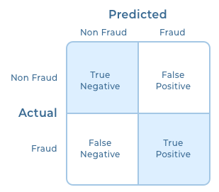
To derive the evaluation metrics, I chose confusion matrix. A confusion matrix compares actual data with predicted data and gives you the number of correct and incorrect classifications. When the model predicts fraudulent claim as fraud, it is a true positive (TP) and if it predicts fraudulent as non-fraud, it is a false negative (FN). Similarly, when the model predicts a non-fraud claim as fraud, it is a false positive (FP) and if it predicts a non-fraud claim as non-fraud, then it is a true negative (TN).
I decided to go ahead with the following metrics:
I decided to go ahead with the following metrics:
Accuracy (How often was the classifier correct?)
Accuracy = (TP+TN)/(TP+TN+FP+FN)
Precision (What proportion of fraud predictions were correct?)
Precision = TP/(TP+FP))
Recall: (Out of the total fraud entries, how many did the model predict?)
Recall = TP/(TP+FN)
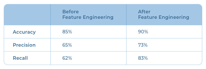
With the metrics finalized, I implemented a simple logistic regression model as it is the easiest method to solve a general classification problem. On evaluation, the model had an accuracy of 85%, precision of 65%, and a recall of 62%. The low performance was due to noise in the dataset. Let me explain how I improved the result by altering some of the features in the dataset.
Feature Engineering and Selection
Feature selection allows you to remove irrelevant or ambiguous features that don’t contribute to the modeling. For example, vehicle age is an important feature in vehicle insurance fraud detection. Claims submitted for older vehicles have a higher probability of being fraud due to their low resale value. However, the postal code of the customer is not that relevant and might end up confusing the model.
New features can also be derived from the raw dataset, in a process called feature engineering, to improve model performance. For example, the dataset I’d chosen had these two features: the date of purchase of the vehicle and the date of the incident that resulted in claim submission. These two features were adversely impacting model performance because of their high variability. I decided to combine these two seemingly irrelevant features to create a new relevant feature called vehicle age. (Note: This is just one type of feature engineering.)
There are proven statistical methods to automate feature selection and engineering. These are some of the methods I used:
- Correlation Coefficient: This is used to measure the correlation between each feature and the target variable. The value ranges from -1 to 1. If it’s close to zero, it indicates that a feature has no impact on the target variable. Thus we can eliminate features that have no role in the training process. Policy number in our dataset is one such example.
- Multicollinearity: This refers to a situation where multiple features give the same insight. In our dataset, we had four features related to claim amount: total claim amount, injury claim, property claim, and vehicle claim. We computed the cross-correlation matrix to detect and remove correlated features. Variance inflation factor (VIF) is another method to do the same.
- Forward Selection and Backward Elimination: We begin with an empty feature set. At each forward step, one feature is added based on predefined criteria and the model performance is evaluated. This is continued till we get the desired performance or all the features are added. This gives us features that are significant for model performance. Backward elimination is the opposite of this process. The modeling process begins with a model trained on a full set of features. During each iteration, a feature that contributes the least to performance is removed.
- Discretization: Converting continuous variables to discrete categories can sometimes improve model performance. Replacing age with age group is an example of such a transformation.
- Principal Component Analysis (PCA): PCA algorithm accepts an existing feature set and returns a new and smaller feature set without losing the information in the original set.
Here’s a before-after comparison of results:
Analysis of Algorithms
We already saw the performance of the logistic regression model on this dataset. I selected four of the common classification algorithms and their variants as well as a neural network-based algorithm for my research.
Decision Trees
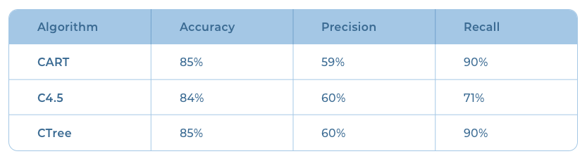
Decision tree algorithms intelligently partition the entire feature set based on decision rules derived from the dataset. Their high interpretability makes them a popular choice. The results obtained with the variants CART, C4.5, and CTree are shown below.
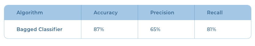
Bagged Classifier
In bagging, also known as bootstrap aggregating, multiple weak models are combined to create a strong model. A bagging algorithm trains multiple versions of a base model (for example, decision tree) by drawing random data samples from the dataset. The predictions from each weak base model (which can be any classification algorithm) are then combined into a final prediction (either by voting or by averaging).
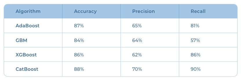
Boosted Classifiers
In a boosting algorithm, the modeling process starts with a weak base model. The boosting process adds new models to the ensemble sequentially to correct the “mistakes” of the previous model. The final prediction is the average of predictions from the individual weak models.
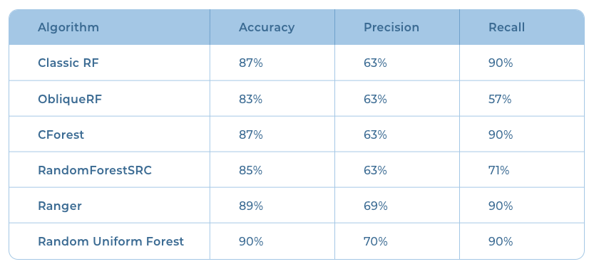
Random Forest
Random forest is a modification of bagged decision trees. In random forest, the base decision trees are not only trained on different data samples but also use a different subset of features. The results from individual trees are then aggregated into the final prediction, similar to bagging. There are different random forest algorithms based on different base models.
Results obtained from random forest variants:
Neural Networks
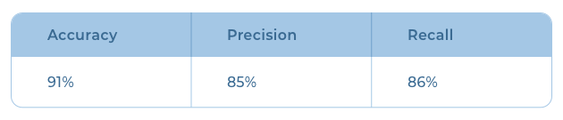
Once I had tested the common statistical models, the obvious way forward was to experiment with neural networks. I developed a custom neural network architecture and trained it with the original dataset without performing any feature selection or feature engineering as the neural network creates features on its own as it learns. The network consisted of SGD optimizer, L1 regularization, drop out, and batch normalization. I decided on the number of hidden layers and units after some parameter tuning. The results were the best in terms of precision and accuracy. The recall was lower though.
Besides the algorithms listed above, I also tried stacking the best performing models in an attempt to further improve the performance. But I could not observe any significant improvement in the results.
I also ran an automated search across multiple base learners (a process known as automated machine learning) to find out the best model, but it couldn’t beat the performance obtained from carefully tuned individual models.
The fraud detection classifier using a custom neural network performed best in my analysis. Among the machine learning models that I tried out, Random Uniform Forest performed the best. Though its accuracy is comparable to that of the neural network model, its precision was only 70%. The result could further be improved by including more examples of fraud data in the dataset.