


Adopting an architecture that meets specific user requirements during setup, you can guarantee optimal performance from your Amazon Redshift cluster. Let us take a look at some of the architectural choices that are available to manage workload and steer clear of outages.
Workload Management (WLM) in Amazon Redshift
When there are several queries from multiple users or multiple sessions, all of them cannot be handled concurrently. Naturally, the later queries will be added to a queue. In Amazon Redshift, the queuing is handled by Workload Management (WLM). There are two WLM modes—automatic and manual.
The two WLM options have their own use depending on the scenario. Automatic WLM is the simpler solution, where Redshift automatically decides the number of concurrent queries and memory allocation based on the workload. There are eight queues in automatic WLM. It comes with the Short Query Acceleration (SQA) setting, which helps to prioritize short-running queries over longer ones. When concurrency scale mode is enabled, Amazon Redshift automatically adds additional clusters for read purposes while the write operation takes place in the main cluster. In manual WLM, there are five queues by default. Up to eight queues can be defined with a maximum concurrency of 50 each. Memory is equally allocated among the queues.
Amazon Redshift uses machine learning algorithms to analyze each query and assign it to a queue. Top priority is assigned to the superuser queue, followed by named queues for specific user groups, and then the default queue.
Defending Against Bad Queries
WLM Query Monitoring Rules (QMR) provide a defense against badly written queries, which may hog resources, making the application unresponsive. For each queue, you can define up to 25 rules, which define metric-based performance boundaries. QMR supports a variety of actions ranging from logging to aborting a query that violates a rule.
Let us now see an example of how we have included various query monitoring rules in a Redshift cluster.
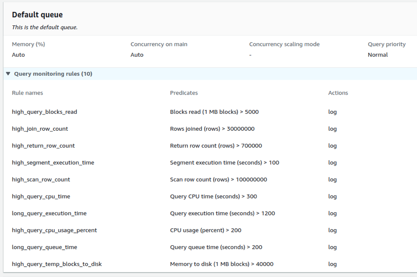
In the above example, only LOG action is used against each rule violation. The rule can be programmatically assigned or set from the AWS management console.
The logs can then be integrated into various platforms such as Slack:
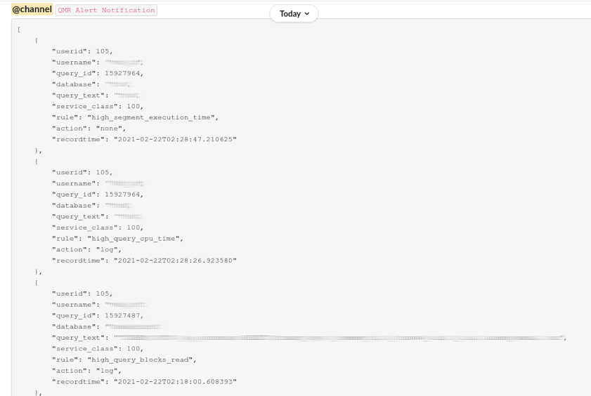
Each log entry provides details of the user, query, and rule violation that triggered the log. Changing various compression encodings and updating table indexes appropriately can lower rule violations. If another team accesses Redshift data with their query and such high_segment_execution_time or high_query_cpu_time are alerted, we could give them a heads-up and suggest how the queries can be made more efficient.
Apart from LOG, there are HOP and ABORT actions. The HOP action (available only in manual WLM) logs the action and hops the query to the next matching queue. The ABORT action creates a log and then aborts the query, except for certain statements and maintenance operations like COPY, ANALYZE and VACUUM. The system tables involved are STL_WLM_RULE_ACTION (when rule predicates are met), STV_QUERY_METRICS (records current running query metrics), and STL_QUERY_METRICS (records completed query metrics).
Workload management is not a substitute for well-designed queries. QMR violations indicate potential areas for query optimization. Analysis of query performance can be helpful in this process. In AWS Management Console, under Redshift Cluster, we can view the details of query performance.
Health status checks can be set up in Amazon Redshift easily using Nagios and Amazon Cloudwatch for alerts when the usage crosses a fixed threshold. These help in the early and fast detection of any network outages and environment problems.

Here the Nagios alert for disk usage has been set for a threshold of 80%. On being alerted of excess usage, we can view the query and all related details that triggered the alert on the console.
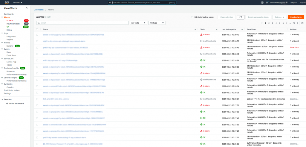
This is a Cloudwatch dashboard where different states like OK, In alarm, Insufficient data, etc., are alerted based on CPU utilization, Memory utilization, and NetworkIn for the instance.
Another option in Redshift that supports performance improvement is the ANALYZE command, which updates the statistical metadata the query planner uses to choose the optimal plan. Maintaining current statistics helps to run complex queries in the shortest possible time. In a similar manner, Amazon Redshift also supports automatic vacuum sort and vacuum delete procedures which sort, physically delete soft-deleted rows, and reclaim space. We can also schedule VACUUM commands during reduced load periods.
Benefits of Using RA3
Amazon Redshift provides different node types:
- Dense Compute DC2 - best for less than 500GB
- Dense Storage DS2 - best for warehousing using HDDs
- RA3 - Instances with managed storage
Compared to ds2 xlarge node type, RA3 with 4 vCPU offers five times more storage capacity for a comparable price. Advantages of RA3 include automatic scaling of storage capacity, higher bandwidth networking that minimizes the time taken for data transfer to and from S3, and you can pay per hour for the compute and separately only pay for the managed storage that you use. And it takes just a few clicks to upgrade your current configuration to RA3. These capabilities allow Redshift to provide three times better performance and storage than any other cloud-based data warehousing service.
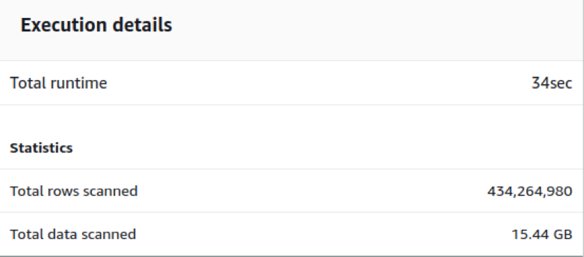
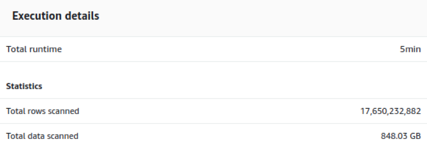
Fig. 5(a) shows the performance of a 16 node ds2.xlarge node type with 32TB storage. We can see that 434 million records with 15 GB data takes 34 seconds for runtime. And the insertion query of 17.65 billion records worth 848 GB takes just 5 minutes for execution (Fig. 5(b)).
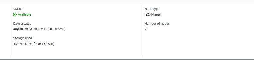
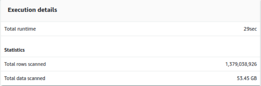
Fig. 6(a) is the configuration of a RA3.4xlarge instance with a compute of 12 vCPU, memory of 96 GiB, and addressable storage capacity of 256 TB, and Fig. 6(b) is an example execution detail from this 2 node RA3 cluster. When we compare the performance of ds2 node Fig. 5(a) with RA3 cluster Fig. 6(b), we see that less time is taken for three times more rows. One billion records worth 53.5 GB has scanning and execution done in just 29 seconds.
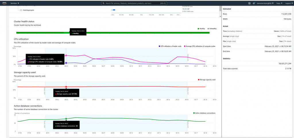
Let us now analyze a query involving 2.13 TB data with more than 58 billion records scanned and multiple operations like union, joins, and aggregations done before the final insertion to the table.
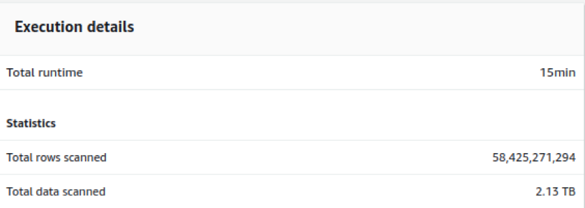
We see that even with such complex operations, CPU utilization rises up to 8-9% while storage used is 68%. An active database connection is 38-45 and the cluster health remains good throughout.
Conclusion
Intelligent automated workload management systems and new architectures like RA3 are enhancing Amazon Redshift’s position as the top-tier data warehousing solution. A variety of monitoring and management solutions on the one hand helps us to optimize the system and on the other hand ensure its continuous availability.